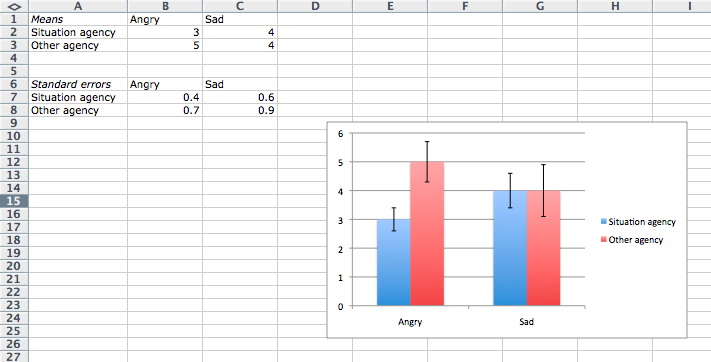
We ran into a problem earlier trying to figure out how to add error bars with a different standard error for each of four bars in a bar graph (Excel calls this a column graph). The way to do this is to set up two tables: one that has your means and another that has your standard errors.

Next, click on one of the sets of bars in the graph. In this case, I’ll click on the situational agency bars (blue bars). Right-click the bars and select “Format Data Series…”.

In the window that opens, select “Both” under Display, select “Cap” under End Style, and click “Custom:” under Error amount. Then click the Specify Value button. You can delete the positive and negative default error values. Then, click in the response box for Positive Error Value after you’ve cleared it and click to highlight the two cells with situational agency standard errors.

Do the same thing for the Negative Error Value. You should have custom standard error bars for the situational agency data. Finally, you can just repeat the same process for the other agency data and you should end up with something like this: